How to Speed-Up Training of Language Models

Language model training is slow, even when your model is not very large. This is because you need to train the model with a large dataset, and there is a large vocabulary. Therefore, the model requires many training steps to converge. However, there are techniques that can speed up training. In this article, you will learn about them. In particular, you will learn about:

• Using optimizers
• Using learning rate schedulers
• Other techniques for better convergence or reduced memory consumption

Let’s get started.

Overview

This article is divided into four parts; they are:

• Optimizers for Training Language Models
• Learning Rate Schedulers
• Sequence Length Scheduling
• Other Techniques to Help Train Deep Learning Models

Optimizers for Training Language Models

Adam has been the most popular optimizer for training deep learning models. Unlike SGD and RMSProp, Adam uses both the first and second moments of the gradient to update the parameters. Using the second moment can help the model converge faster and more stably, at the expense of increased memory usage.

However, when training language models nowadays, you typically use AdamW, the Adam optimizer with weight decay. Weight decay is a regularization technique to prevent overfitting. It usually involves adding a small penalty to the loss function. But in AdamW, weight decay is applied directly to the weights. This is believed to be more stable because the regularization term is decoupled from the calculated gradient. It is also more robust to hyperparameter tuning, as the regularization term is applied explicitly to the weight update.

In formula, the AdamW weight update algorithm is as follows:

$$
\begin{aligned}
g_t &= \nabla_\theta L(\theta_{t-1}) \\
m_t &= \beta_1 m_{t-1} + (1 – \beta_1) g_t \\
v_t &= \beta_2 v_{t-1} + (1 – \beta_2) g_t^2 \\
\hat{m_t} &= m_t / (1 – \beta_1^t) \\
\hat{v_t} &= v_t / (1 – \beta_2^t) \\
\theta_t &= \theta_{t-1} – \alpha \Big( \frac{\hat{m_t}}{\sqrt{\hat{v_t}} + \epsilon} + \lambda \theta_{t-1} \Big)
\end{aligned}
$$

The model weight at step $t$ is denoted by $\theta_t$. The $g_t$ is the computed gradient from the loss function $L$, and $g_t^2$ is the elementwise square of the gradient. The $m_t$ and $v_t$ are the moving average of the first and second moment of the gradient, respectively. Learning rate $\alpha$, weight decay $\lambda$, and moving average decay rates $\beta_1$ and $\beta_2$ are hyperparameters. A small value $\epsilon$ is used to avoid division by zero. A common choice would be $\beta_1 = 0.9$, $\beta_2 = 0.999$, $\epsilon = 10^{-8}$, and $\lambda = 0.1$.

The key of AdamW is the $\lambda \theta_{t-1}$ term in the gradient update, instead of in the loss function.

AdamW is not the only choice of optimizer. Some newer optimizers have been proposed recently, such as Lion, SOAP, and AdEMAMix. You can see the paper Benchmarking Optimizers for Large Language Model Pretraining for a summary.

Learning Rate Schedulers

A learning rate scheduler adjusts the learning rate during training. Usually, you would prefer a larger learning rate in the early training steps and reduce it as training progresses to help the model converge. You can add a warm-up period to increase the learning rate from a small value to its peak over a short period (typically 0.1% to 2% of total steps), then decrease it over the remaining training steps.

A warm-up period usually starts with a near-zero learning rate and increases linearly to the peak learning rate. A model starts with randomized initial weights. Starting with a large learning rate can lead to poor convergence, especially for large models, large batch sizes, and adaptive optimizers.

You can see the need for a warm-up from the equations above. Assuming the model is uncalibrated, the loss may vary significantly across subsequent steps. Then the first and second moments $m_t$ and $v_t$ will be fluctuating greatly, and the gradient update $\theta_t – \theta_{t-1}$ will also be fluctuating greatly. Hence, you would prefer the loss to be stable and move slowly so that AdamW can build a reliable running average. This can be easily achieved if $\alpha$ is small.

At the learning rate reduction phase, there are a few choices:

• cosine decay: $LR = LR_{\max} \cdot \frac12 \Big(1 + \cos \frac{\pi t}{T}\Big)$
• square-root decay: $LR = LR_{\max} \cdot \sqrt{\frac{T – t}{T}}$
• linear decay: $LR = LR_{\max} \cdot \frac{T – t}{T}$

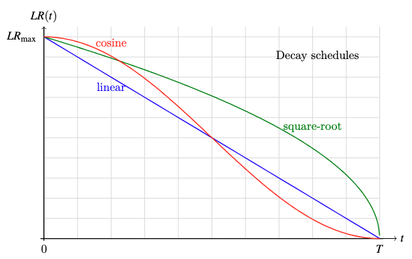
Plot of the three decay functions

A large learning rate can help the model converge faster, while a small learning rate can help the model stabilize. Therefore, you want the learning rate to be large at the beginning when the model is still uncalibrated, but small at the end when the model is close to its optimal state. All decay schemes above can achieve this, but you would not want the learning rate to become “too small too soon” or “too large too late”. Cosine decay is the most popular choice because it reduces the learning rate more slowly at the beginning and maintains a lower learning rate toward the end, which are desirable properties to help the model converge faster and stabilize, respectively.

In PyTorch, you have the CosineAnnealingLR scheduler to implement cosine decay. For the warm-up period, you need to combine with the LinearLR scheduler. Below is an example of the training loop using AdamW, CosineAnnealingLR, and LinearLR:

Running this code, you may see:

Notice how the learning rate increases and then decreases. Note that term eta_min=min_lr in the cosine scheduler above. The default value is 0; it is only a parameter used to calculate the learning rate. You can set it to approximately 0.1%- 1% of the peak learning rate.

Sequence Length Scheduling

Language models are trained with sequence data. Transformer models or recurrent neural networks are both architecturally agnostic to the sequence length. However, you may want to train the model on a long sequence to help it learn to handle long context.

In training, long sequence lengths can be problematic. First, you train on batches of sequences, and ragged lengths mean you need to pad the sequences to the batch’s maximum length. While you ignore padded tokens, your model still needs to process them, wasting resources. Second, in the attention mechanism, the complexity is quadratic to the sequence length. The longer the sequence, the more costly it is to process.

Therefore, you may want to create batches with sequences of similar length to avoid excessive padding. This is known as sequence packing.

You may also want to train the model with shorter sequences first. You can accelerate training by forcing the model to learn language patterns with shorter sequences. Once the model has fairly converged, you can gradually increase the sequence length to help the model learn how to handle long contexts. However, you still want to use short sequence lengths intermittently to make sure the converged model can handle both long and short sequences equally well.

These are common techniques in training large language models to save computational resources. Note that you still set the model’s maximum sequence length to a fixed value, which affects how you configure the positional embeddings. However, you do not exhaust the maximum sequence length until the model has fairly converged.

Implementing sequence-length scheduling requires writing a more complex data loader that accounts for the current epoch to return the appropriate training data.

Other Techniques to Help Train Deep Learning Models

Random Restart

Training a deep learning model is a complex process and not easy to get right, especially for large models. One common issue is the model getting stuck in a local minimum and being unable to converge. Using momentum in gradient descent can help the model escape from local minima, but is not always effective. Another approach is to simply restart training if you observe the model failing to converge.

Random restart is a training strategy in which the model is trained multiple times from scratch. It uses different random seeds each time, so the model starts with different initial weights and a different data shuffle. This is done to help you avoid getting stuck in the same local minimum, so you can pick the one with the best performance. This is ideal if you can train multiple models for fewer epochs initially, then select the best model from the pool to complete training with more epochs.

Gradient Clipping

One common issue in training deep learning models is gradient explosion. This is especially common if you train the model using lower-precision floating-point numbers, in which the range of the gradient could be too large to be represented. Gradient clipping is the technique of limiting the magnitude of the gradient to a safe value. Without it, you may see your training process suddenly fail due to the model weights or loss function becoming NaN or infinity.

There are multiple ways to clip gradients. The most common approach is to clip the gradient so that the L2 norm is below a safe threshold, such as 1.0 or 6.0. You can also clip the gradient to a value range, such as -5.0 to 5.0.

Gradient clipping by L2 norm means scaling the entire gradient vector if the L2 norm $\Vert g_t \Vert_2$ is greater than a safe value $c$:

$$
\hat{g_t} = \min\big(1, \frac{c}{\Vert g_t \Vert_2}\big) \cdot g_t
$$

On the other hand, gradient clipping by value means setting the gradient to a safe value whenever the gradient exceeds that value:

$$
\hat{g_t} = \begin{cases}
-c & \text{if } g_t < -c \\
g_t & \text{if } -c \le g_t \le c \\
c & \text{if } g_t > c \\
\end{cases}
$$

Using gradient clipping in PyTorch is straightforward. You can use the torch.nn.utils.clip_grad_norm_ function to clip the gradient by L2 norm, or the torch.nn.utils.clip_grad_value_ function to clip the gradient by value. Below is an example:

Should you use gradient clipping by norm or by value? Clipping by value imposes a hard limit on individual gradients and unevenly changes their magnitudes. If some gradients are naturally larger, you make learning imbalanced across different layers of your model. This will disrupt the natural flow of information during training and may lead to suboptimal training. On the other hand, clipping by norm scales everything equally. If the gradients are highly imbalanced, scaling them down will artificially introduce vanishing gradients in your training.

Mixed Precision Training

When a model becomes too large, memory consumption becomes a bottleneck as well. You may want to save memory by using lower-precision floating-point formats during training, such as half-precision (float16) or bfloat16. Compared with single precision (float32), float16 and bfloat16 can reduce memory consumption by half, but at the cost of reduced range and precision.

Therefore, you may want to use mixed precision training, in which part of the model uses float32 while the other part uses float16. A common choice is to use float32 for biases but float16 for weights in linear layers.

Modern GPUs can run float16 operations at the same speed as float32, but since you can operate on more data at the same time, you can effectively run the training process at double speed.

Regularization

In AdamW optimizer above, you have a parameter $\lambda$ to set the strength of weight decay. The default value in PyTorch is 0.01. However, if you are resource-constrained, you may want to use fewer training steps and larger learning rates. But the consequence is that the converged model would be biased. You can improve the model’s generalization by using a stronger weight decay factor to compensate for the shorter training horizon.

Further Readings

Below are some resources that you may find useful:

Summary

In this article, you learned about some techniques to speed up the training process of deep learning models, especially for large language models. Specifically, you learned that:

• AdamW with cosine decay is the most popular optimizer and learning rate scheduler for training language models.
• You can use sequence length scheduling to save computational resources when training language models.
• Techniques like random restart and gradient clipping can help you train the model more stably.
• Mixed precision training can help you reduce memory consumption.